Kaushik Gopu joined the team

UNC Charlotte Computer Science graduate student Kaushik Gopu joined the IGB application development team in May of 2023.

Since joining the team, he has been working on adding new features to Integrated Genome Browser and on updating the IGB App called ProtAnnot. He also has contributed to improving our use of OSGi frameworks, by trying out and reviewing various on-line tutorials discussing declarative services annotations and their use.

In only a month, you’ve contributed a lot. Keep up the good work!

Adding a Sorghum version 2.0 genome assembly to IGBQuickLoad

Recently, a researcher working with the sorghum genome posted this question on BioStars – Question: IGB- genome sequence in sequence viewer just shows dashes

Updating to a more recent version of IGB solved the problem, but the question reminded me that Phytozome had released a new sorghum assembly and that we needed to update the IGBQuickLoad site.

In this post, I’ll describe how I updated IGB to the latest sorghum genome assembly using data from Phytozome and a few easy-to-use command line tools.

Step One. Get the data

To start, Nowlan downloaded gene annotations, sequence, and a gene information file from Phytozome.net. The files were:

  • Sbicolor_255_v2.0.fa.gz – sequence data
  • Sbicolor_255_v2.1.gene_exons.gff3.gz – gene models
  • Sbicolor_255_v2.1.defline.txt – gene information file, summarize function

He put them in our shared IGB Dropbox, saving me the trouble of logging in and figuring out where to look. Thank you Nowlan!

Step Two. Find out when the genome was released and what it’s called.

Using Google searches, I found a page describing the new assembly and associated gene annotations. The genome assembly is called “version 2.0” and the annotations are called “version 2.1.”

A search for “Sorghum 2.0 released” found this news page which contained text:

[07 Jun 2013]   v2.1 of Sorghum bicolor now available as early release.

This new item refers to the genome annotations, not the genome assembly, but probably the two were released about the same time, so I decided to use this. Why does it matter? It matters because including the month and year in the name of a genome release tells us which release is most recent. This is why IGB gives every  assembly a name that tells it (and us) how old the genome is.

Step Three: Check out a copy of IGBQuickLoad.

We are using subversion (a version control system) to track and distribute files that are part of the IGBQuickLoad site.

To add the new data to IGBQuickLoad, I first have to check out a copy using svn. (For more information about svn, see: http://svnbook.red-bean.com/.)

svn co https://svn.transvar.org/repos/genomes/trunk/pub/quickload

I’ve configured my computer to provide the correct user name and password when I execute svn commands. Otherwise, I would need to supply my user name and password uisng the –username and –password options. For more information, run

svn co -h

Step Four: Add new directory for this new genome

Following IGB conventions, I added a new directory to the IGBQuickLoad data repository using svn:

svn mkdir S_bicolor_Jun_2013

By convention, we keep genome assembly data files and meta-data files in a directory named after the species and release date.

I also added new lines to the .htaccess and contents.txt files:

htaccess:

AddDescription "Sorghum bicolor v. 2.0" S_bicolor_Jun_2013

This ensures the directory listing on the IGBQuickLoad.org Web site will report the version name and species.

contents.txt:

S_bicolor_Jun_2013      Sorghum bicolor v2.0 (June 2013)

This ensures IGB will list the genome in the Current Genome tab. When IGB first accesses an IGBQuickLoad site, it fetches this “contents.txt” file and uses it to determine the names and locations of genome assemblies available on the site.

This contents.txt file is a tab-delimited file with two columns – the first column lists genome directories and the second column lists the human-friendly name of the genome, which is what IGB displays in the IGB window title bar when users selects that genome. Note that sometimes two sites could contain different text in the second genome, but this won’t break IGB. IGB will just show the data from whichever file it read first. So far, this has not posed any problems.

Step Five. Make 2bit sequence file.

I used Jim Kent’s faToTwoBit program to convert the fasta sequence file to 2bit. This format is more compact than fasta and is also random access, which means IGB can use the file to retrieve small parts of the genome quickly when users click the Load Sequence button. By convention, we name the 2bit file after the genome version – this ensures IGB will be able to find it on the site.

faToTwoBit Sbicolor_255_v2.0.fa S_bicolor_Jun_2013.2bit

The fasta file is 702 Mb (almost 1 Gb!) and the 2bit file was only 173M. Much better!

This file must reside in the genome directory S_bicolor_Jun_2013. Because it is not very big, I used svn to add it to the repository.

Step Six. Make genome.txt file.

To populate the Current Sequence tab, IGB needs a “genome.txt” file that lists chromosomes and their sizes – this file, like the 2bit file, resides the in the genome directory. To make this, I use twoBitInfo, another Jim Kent program:

twoBitInfo S_bicolor_Jun_2013.2bit genome.txt

IGB’s Current Sequence table will list the chromosomes in the same order they appear in this file, so I view the first few lines of the file to make sure the most useful (fully assembled) chromosomes appear first in the list:

Chr01   73727935
Chr02   77694824
Chr03   74408397
Chr04   67966759
Chr05   62243505
Chr06   62192017
Chr07   64263908
Chr08   55354556
Chr09   59454246
Chr10   61085274
super_10        8818317

This looks fine. But if it didn’t I might re-order the listing by sequence size:

sort -k2,2nr genome.txt > tmp
mv tmp genome.txt

Step Seven. Make annotations meta-data file (annots.xml)

Here, I used a program named phytozomeGff3ToBed.py, available from a Loraine Lab git repository. This program converts GFF to BED12 format:

phytozomeGff3ToBed.py -g Sbicolor_255_v2.1.gene_exons.gff3.gz -b tmp.bed

I used a Unix one-liner convert the BED12 file to BED-detail format, sort the file by sequence name and gene model start position, compress it using bgzip, and then save the result to a new file named for the genome version:

bedToBedDetail.py -g Sbicolor_255_v2.1.defline.txt -b tmp.bed | sort -k1,1 -k2,2n | bgzip > S_bicolor_Jun_2013.bed.gz

To share reference gene model annotations, we use BED-detail format.  It’s compact and more convenient for data analysis than GFF3. It contains all the usual field in a BED12 file, plus two extra fields. In IGB, our BED-detail files

  • report locus names in field 13, useful for grouping alternative transcripts arising from the same transcriptional unit
  • don’t use the itemRGB field (we don’t color-code gene models, but we might do that someday)
  • insert the start position in the thickStart and thickStop fields when a gene model doesn’t encode a protein

When we distribute annotations file, we also index them using tabix, which requires that the indexed file be sorted and block compressed using bgzip. (Google “tabix” to find a copy – it’s open source and associated with the samtools package.)

To index the file using tabix, I did this:

tabix -s 1 -b 2 -e 3 S_bicolor_Jun_2013.bed.gz

This created a file named S_bicolor_Jun_2013.bed.gz.tbi (“tbi” for tabix index) which must reside in the same directory as its corresponding data file for IGB (or other programs) to use it. The index file enables IGB to quickly load the file or retrieve just parts of it via byte-range queries.

Next, I viewed the first few lines of the file:

Chr01    24317    38116    Sobic.001G000400.2    0    -    24631    36898    19    590,255,172,228,134,84,291,333,107,126,166,104,161,901,91,291,85,83,3870,683,1377,1661,2230,8581,8772,9179,9608,9929,10147,10436,10651,10922,11953,12118,12497,13040,13412,    Sobic.001G000400    similar to PDR-like ABC transporter
Chr01    24317    42528    Sobic.001G000400.1    0    -    24631    42234    20    590,255,172,228,134,84,291,333,107,126,166,104,161,901,91,291,85,83,121,500,    0,683,1377,1661,2230,8581,8772,9179,9608,9929,10147,10436,10651,10922,11953,12118,12497,13040,17387,17711,    Sobic.001G000400    similar to PDR-like ABC transporter
Chr01    50023    50488    Sobic.001G000500.1    0    -    50037    50488    54,263,    0,202,    Sobic.001G000500    Not Available
Chr01    53429    60786    Sobic.001G000600.1    0    -    60555    60738    204,419,    0,6938,    Sobic.001G000600    Not Available

This looked good. Field 4 contained gene model name, field 13 contained locus name, and field 14 contained a description taken from the gene information file (Sbicolor_255_v2.1.defline.txt), but reported “Not Available” when nothing about that gene was listed.

How many gene models have no information?

gunzip -c S_bicolor_Jun_2013.bed.gz | grep -c "Not Available" 
   14622
gunzip -c S_bicolor_Jun_2013.bed.gz | wc -l
   39441

Out of 39,441 gene models, around 14,000 had no functional information. This isn’t great, but it’s not unusual for a newly annotated genome.

Step Eight. Make a HEADER.html file – documentation

Next, I created a HEADER.html file that documents the files and where they came from. When user visit the new genome directory on the web, they’ll see the HEADER file contents displayed along with a listing of the files.

Step Nine. Make an annots.xml file

To ensure that IGB will show the genome, I next needed to add an “annots.xml” meta-data file that reports the data sets that are available for the genome. Because I’m a little lazy, I use the “svn cp” (svn copy) command to make an annots.xml file using the file from a previous genome version.

svn cp ../S_bicolor_Jan_2009/annots.xml .

I used a text editor to update the data for this new genome:

<files>
  <file name="S_bicolor_Jun_2013.bed.gz" 
        title="Genes"
        description="Version 2.1 gene models from Phytozome, Nov. 2014."
        url="S_bicolor_Jun_2013"
        foreground="000000"
        name_size="14"
        direction_type="arrow"
        background="FFFFFF"
        load_hint="Whole Sequence"
        show2tracks="true"
  />  
</files>

What all this means:

  • name – name of the file in the file system; IGB assumes it resides in the same directory as the annots.xml file, inside the genome directory S_bicolor_Jun_2013
  • title – name IGB gives this data set in the Available Data sets section of the Data Access tab. This is also the name IGB displays in the track label once the data are loaded into a track.
  • description – displayed as a tooltip when users position the cursor over the “i” icon next to the data set under Available Data Sets.
  • url – if users click on the “i” icon, a Web browser will open to this location relative to the IGBQuickLoad root directory. (http://www.igbquickload.org/quickload/S_bicolor_Jun_2013 in this case.)
  • foreground – annotation color
  • name_size – font size for the track label
  • background – background color for the track
  • load_hint – how and when to load the data. “Whole Sequence” means: load all the data at once.
  • show2tracks – whether or not to divide the annotations into two tracks – one for minus strand genes and another for plus strand genes

Step Ten. See how it looks in IGB.

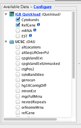
For testing and development, I’ve been adding and updating the files in a local copy of the IGBQuickLoad repository that I’ve checked out onto my computer. To see how the new files will look in IGB, I use the Data Sources tab in the Preferences window to add the local QuickLoad site to IGB.

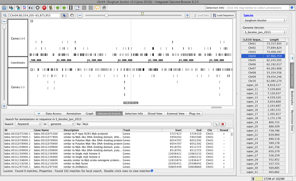
Then, I used the Current Sequence tab to select species Sorghum bicolor and genome version S_bicolor_Jun_2013. I also ran a quick keyword search (Advanced Search tab) to make sure the “details” part of the BED-detail file is read correctly into IGB.

Everything looks good!

S_bicolor

Step Eleven. Check it into the repository and update the public IGB QuickLoad sites.

I then used “svn add” and “svn commit” to add the new files to the repository. Then I logged into the main IGBQuickLoad site and the IGBquickLoad backup site and ran “svn up” to add new files and update old ones.

This entire process, including writing this post and coffee breaks, took about two hours of my time.


Farewell Tarun

Yesterday we had a lab dinner to celebrate Tarun Kanaparthi’s December 2014 graduation – he is earning his Masters degree in Computer Science from UNC Charlotte.

Following a vacation, he plans to start work at his new job, to be determined. Like many recent or soon-to-be graduates in computer science and bioinformatics, he is trying to decide between multiple opportunities. It’s nice to know that computer programming and data analysis skills are still in demand. Congratulations Tarun!

Here is a photo from the going-away party. From left to right, we are:

April Estrada, Ivory Blakley, Mason Meyer, David Norris, Tarun Kanaparthi, Tarun Mall, Nowlan Freese

IMG_1541

Using Table Browser at UCSC to get a data set for IGB

The UCSC Genome Bioinformatics site offers a wealth of data from many genomes, ranging from tiny (but deadly) genomes like ebola virus to much larger genomes like our own human genome. Indeed, the reference genome sequence and gene model data sets for many of the genomes the IGB teams hosts on the IGBQuickLoad.org data repository site are originally from UCSC. Other projects – like Galaxy – also rely on UCSC for core data sets. If you have used Galaxy, you may have noticed that Galaxy has built-in genomes for many animal species; these data were imported from the UCSC ecosystem.

When you visit a UCSC-supported genome in IGB, you’ll see a folder named “UCSC (DAS)” in the Available Data Sets  section of the Data Access Panel. If you open the folder, you’ll see many data sets with seemingly cryptic titles – like “nestedRepeats” and “altLocations.” These names correspond to tables in the UCSC database. If you select these data sets and click Load Data in IGB, these data will flow from the UCSC system’s Distributed Annotation Server into IGB.

DAS4HumanHowever, for technical reasons, the UCSC DAS site can only support some of their data sets. To view UCSC data that are not supported in their DAS site, you can use the UCSC Table Browser to download them onto your computer and open them in IGB.

In this post, I’ll explain how you can use the UCSC Table Browser to obtain and then open data sets in Integrated Genome Browser. I’ll also explain how you can use tabix and bgzip to compress and index files that are too large to load into IGB all at once.

Part I: Getting data from the UCSC Web site

In this example, I’ll show you how to get human variation data (SNPs) from the UCSC Web site.

  1. Go  to http://genome.ucsc.edu
  2. Click Tables (top of page)

Configure the browser to access the latest (as of this writing) human genome assembly:

  1. clade Mammal
  2. genome Human
  3. assembly Dec 2013 (GRCh38/hg38) (the latest)
  4. group Variation
  5. track Common SNPs(141)
  6. table snp141Common
  7. region genome
  8. output format BED – browser extensible data
  9. file type returned gzip compressed

Enter a name for the output file – e.g., snp141Common.hg38.bed.gz. It should end with “.gz” to ensure your computer will recognize it as a gzip-compressed file.

Tip: Click the button Describe Table Schema to see what data are in the table.

SNPTableBrowser

to be continued

Adding new fruit fly annotations to QuickLoad (by Ann)

Several IGB users asked us to add the latest fruit fly genome and annotations to IGB. Here I describe how I did this, using data files downloaded from FlyBase, the chief annotation authority for fruit fly genomes.

In July 2014, FlyBase and Berkeley Drosophila Genome Project (BDGP) released a new genome assembly for the fruit fly genome Drosophila melanogaster. They also released a new set of gene model annotations in various formats – including GFF, GTF, and XML.

To make the data available to IGB users, I needed to download the sequence data and reference gene model annotations, convert them to formats IGB can use for visualization, and then deploy the converted files on the IGBQuickLoad.org Web site. This is the Web site that IGB uses to retrieve data for annotated, sequenced genomes. When IGB users select a genome, the reference gene model track data that automatically loads into IGB comes from the IGBQuickLoad site or one of its mirror sites.

Adding a new genome directory to the IGBQuickLoad data repository

To start, I added a new genome version directory (folder) to the IGBQuickLoad.org data repository. I did this using “svn”, the program we use to manage the data sets. I used the “svn mkdir” command to create a new directory named D_melanogaster_Jul_2014, following our naming convention for genome versions. In IGB, we use the genus, species, release month and year to specify a genome version. (Sometimes we also include an extra name to indicate variety or something else, such as  Z_mays_B73.) However, in this case, we don’t need a variety suffix, so we only use the genus and species to indicate the genome.

The IGBQuickLoad.org data repository is version-controlled as part of a large subversion (svn) repository – the master copy is hosted at https://svn.transvar.org/repos/genomes/trunk/pub/quickload/ and is publicly accessible. Which means: anyone who wants a copy can use “svn co” to get it.

The IGB team has been using subversion for many years to track important data files, like gene annotations or sequence, that people use for data analysis and visualization in IGB. To save effort, we also use the same repository to serve data files to IGB, using the IGB QuickLoad mechanism. When we need to deploy a new quickload site – on our local computers or via a Web server – we just use “svn co” to check out a fresh copy and then copy over some bigger data files (e.g., BAM files) that are too large to add to the repo. However, genome sequence files for smaller genomes (like fruit fly) are not very large and so I usually version-control these in the repository along with the gene model files. (More on this later.)

Adding genome sequence to the repository

Next, I looked around the FlyBase.org Web site to find a file containing the new genome assembly sequences. I found it here: ftp://ftp.flybase.net/genomes/Drosophila_melanogaster/dmel_r6.03_FB2014_06/fasta/. The directory contained a file named dmel-all-chromosome-r6.03.fasta.gz. Based on the name, I guessed this file contained the genome sequence, so I downloaded that.

Next, I used Jim Kent’s faToTwoBit program to convert the file from fasta to 2bit format, a compressed, indexed format that enables IGB (and other programs) to retrieve data from the file without having to read the entire thing – called “random access.” This is what enables IGB to load just part of a genomic sequence, which is faster and more memory-efficient than loading the entire thing.

After converting the fasta file to 2bit, I next used Kent’s twoBitInfo program to make a genome.txt file, which is a tab-delimited file that lists the sequences and their sizes. When a user selects a genome version in IGB, IGB then sends a request to a QuickLoad site that supports that genome, asking for a copy of that genomes genome.txt file, which is stored in the genome directory for that genome version. IGB reads this file and uses the information to populate the Current Sequence tab on the right side of the main IGB  window. The Current Sequence tab displays a sortable, clickable table that you can use to change chromosomes in the main display.

This is different from (and we think better than) other genome browser designs, where users have to operate a menu or click on a to-scale genome graphic to change which sequence is on display. Menus don’t work well if there are more than a few items in the menu, and a to-scale genome graphic is even worse because smaller contigs are too hard to select. That’s why in IGB, we use a sortable table instead. And, of course, users can also search for contigs and genes by name.

A quick review of the genome.txt file revealed that this new assembly contains the expected fruit fly chromosome arm sequences (e.g., 2L), but it also contains a lot of other sequences with identifiers like “211000022280328” and “2Cen_mapped_Scaffold_10_D1684.” Altogether, the genome sequence file contains 1,870 sequences.

Interesting! I was not expecting to find so many sequences in this release because the previous release (dm3) contained the autosomal chromosome arms and the sex chromosomes only. But including these additional sequences makes sense. I imagine that the assembly creators at BDGP did not want to omit some-one’s favorite gene from the release just because it didn’t assemble into the main chromosome arms.

Getting gene model annotations from FlyBase

Looking around a bit more, I found these two folders: ftp://ftp.flybase.net/genomes/Drosophila_melanogaster/dmel_r6.03_FB2014_06/gtf/ and ftp://ftp.flybase.net/genomes/Drosophila_melanogaster/dmel_r6.03_FB2014_06/gff/.

I reviewed the files in each folder, starting with the GFF files. I’ve never had good experiences with GFF, mainly because different people use it in difference ways, despite many attempts to standardize the format. At first glance, the FlyBase GFF looked too complex to handle easily.

So next, I turned to the files in the GTF directory. I don’t know why FlyBase included these files in their ftp site, but I’m guessing it had something to do with supporting users who want to use CuffLinks to analyze RNA-Seq data. CuffLinks uses GTF to represent gene models, andI already have code that converts CuffLinks GTF to BED-detail, our preferred format for distributing gene model data files in IGB. A quick review of the file showed me that the format was indeed simpler, and so I decided to work with that file instead of the GFF files.

Unfortunately, my Cufflinks GTF conversion code failed on the FlyBase GTF file because it lacked transcript features. Also, FlyBase included many in-line comments.

Nonetheless, it looked simpler, and so I wrote a new script to handle FlyBase GTF as distinct from other forms of GTF. The script is named flybaseGtfToBed.py and resides in bitbucket repo https://bitbucket.org/lorainelab/genomes_src. I used this new code to create a BED-detail file named D_melanogaster_Jul_2014.bed, which contains gene models converted from the GTF file.

About BED-detail and how we use it in IGB

BED-detail, also known as BED14, has all the same fields as BED12, plus two more. In IGB, we use these extra fields to provide useful meta-data about a gene model. In IGB, field 13 contains the gene name for a gene model. And field 14 contains human-friendly text describing the gene’s function. When users open these files in IGB, IGB formats them internally in a way that allows users to do keyword searches on field 14. This is very useful, but of course it depends on having human-friendly text available to use in this field. For Arabidopsis, we use the “curator summary” text in field 14. I’m not sure what we can use for fruit fly as I have not been able to find an equivalent to the Arabidopsis “curator summary.”

BED-detail benefits in other areas – high-throughput data analysis

We use BED-detail mainly because it’s compact and easy to index using tabix. (More on this later.) Also, the structure of the BED-detail files makes them extremely useful in high-throughput data analysis using R/Bioconductor tools. My favorite RNA-Seq data analysis trick to find the smallest start and largest end position for all transcripts belonging to the same gene, and I identify those by grouping on gene symbol. Then I use the coordinates to count reads overlapping the gene. Once I have those counts, I can feed them to edgeR or DESeq or other similar tools.

Deploying the new gene model BED-detail file on IGBQuickLoad

For simplicity, I named the file after the genome release: D_melanogaster_Jul_2014.bed. Next, I sorted the file by sequence name and start position, compressed it using bgzip, indexed it using tabix, and added the files to our subversion repository:

sort -k1,1 -k2,2n D_melanogaster_Jul_2014.bed | bgzip > D_melanogaster_Jul_2014.bed.gz
tabix -s 1 -b 2 -e 3 D_melanogaster_Jul_2014.bed.gz
svn add D_melanogaster_Jul_2014.bed.gz.*
svn ci -m "Converted from FlyBase GTF using flybaseGtfToBed.py"

Adding meta-data file: annots.xml and HEADER.html

to-do

Viewing the data in IGB

Here’s an image from IGB showing an alternatively spliced gene (para) from chromosome X. The depth graph made from the gene models (FlyBase) track highlights differentially spliced regions. Places where the depth graph changes height indicate alternative splicing.

DmelX

Moving genomes source code to bitbucket (by Ann)

Today I’m moving source code (mainly python) from the genomes subversion repository over to a new repository on BitBucket.

The genomes subversion repository contains version-control data files for many different genomes that we’ve collected from many sources, such as the UCSC Genome  downloads page, the UCSC Table Browser, Phytozome (for plants), and model organism databases like DictyBase. We launched the genomes repository back in 2008 as part of an Arabidospis 2010 project grant that support IGB from 2008 to 2012. Our original idea was to use version control systems (cvs or svn) to track big data files from Arabidopsis and other species. The repository would not only serve as a useful data archive, it would also provide a way to feed data into IGB.

However, the genomes repo also contains source code we wrote for converting data files, setting up QuickLoad sites, and other tasks. The source code was stored in a directory named “src” (for “source”). You can browse it here: https://svn.transvar.org/repos/genomes/trunk/pub/src/.

Today, I’m moving all that source code over to a new repo hosted on BitBucket: https://bitbucket.org/lorainelab/genomes_src.

I’m doing this because the BitBucket UI for browsing code, reviewing changes, and managing the project is about a thousand times better than what we are currently using on our subversion server. Since BitBucket offers free source code hosting for reasonably sized repositories, there’s no point in hosting any of our source code ourselves, and during the last year, I’ve been happily migrating all our lab code onto BitBucket. Also, I’d like to start using git for version control, at least for all our source code. Setting up a git repository on our server would probably not be difficult, but then we would have yet another service to maintain.  Rather than try to host everything we do on our own machines (which consume electricity and sysadmin time) I’ve realized we should off-load as much as we can onto public, free resources like BitBucket. And at least for now, BitBucket seems like the best option because it’s run by Atlassian, which seems like it has staying power, a mature management structure, and excellent support.

More about the genomes repository:

The genomes repo contains a lot of data, not just code. In fact, most of is data – more than 11 Gb worth of sequence files, annotation files, and some meta-data files describing what’s there.

I’d love to migrate the data onto BitBucket and start using git and not svn for managing the data. I’d love to make it possible for people to fork the repo, improve the annotations, and then issue pull requests back to the main site. The problem is: I don’t know if BitBucket can handle a repository as big as ours – it’s 11 Gb. Also, most of our files are in binary formats (2bit, .tbi, .gz, etc) and I’m not sure how git will handle those files when I or other people make a change. Will it store multiple copies of an enormous file if I modify a small part of it? How would diffs work? It would be terrific if git could somehow handle our binary formats in a smart way.

So for now, I’ll continue to use our subversion server to host and version control the data sets, but I’ll use bitbucket for source code, which is probably what the team at Atlassian would prefer.

One last comment: For now, I’m leaving the “src” directory untouched in the original genomes repo, but I’ll add a notice letting users know that this part of the repository is moving to bitbucket.

Welcome to our blog

Thanks to funding from public sources (NSF, NIH, North Carolina) we get to do interesting research that benefits many people. In this blog, we plan to share some what we’ve learned.

Check back here to read posts on research and related topics from Loraine Lab members.